Score-based models

This post builds on the ideas presented in the video and the accompanying paper blog.

TL;DR; A score-based model is built to estimate $p(x)$ by using the score function. For any input point in the data space, the model predicts its score, which indicates the direction to higher probability (understanding the score function’s meaning is key). Inference uses Langevin dynamics sampling, iteratively applying the model (ideally many times) to move the input towards higher probability areas, resulting in a final sample from the highest probability area.

Recall that we still have problem on $Z_{\theta }$.

Score function

Instead of modeling the density function directly, we model the score function. The score function of a distribution $p(x)$ is defined as

$${\nabla }_{\mathbf{x}}\log p(\mathbf{x})$$

Our model aims to estimate this quantity by approximating

$${\mathbf{s}}_{\theta }(\mathbf{x})\approx {\nabla }_{\mathbf{x}}\log p(\mathbf{x})$$

an approach known as a score-based model. After that we do some math to get

$$\begin{array}{r}{\mathbf{s}}_{\theta }(\mathbf{x})={\nabla }_{\mathbf{x}}\log p_{\theta }(\mathbf{x})=-{\nabla }_{\mathbf{x}}{f}_{\theta }(\mathbf{x})-\underset{=0}{\underbrace{{\nabla }_{\mathbf{x}}\log Z_{\theta }}}=-{\nabla }_{\mathbf{x}}{f}_{\theta }(\mathbf{x}).\end{array}$$

Note that ${\mathbf{s}}_{\theta }(\mathbf{x})$ is independent of the normalizing constant $Z_{\theta }$, which is highly advantageous.

Score matching

The score function, ${\nabla }_{\mathbf{x}}\log p(\mathbf{x}),$ , clearly indicates the direction in which the data probability increases, in other words, score function can tell you for any point in your data space in which direction you have to move to get closer to actual data points (probability increase)

In case of images we can start with random Gaussian image and score will tell you which direction we should move to get closer to image manifold (target image).

To do that we just train score-base model to minimize model and the data distribution:

$$\frac{1}{2}{\mathbb{E}}_{p(\mathbf{x})}[||{\nabla }_{\mathbf{x}}\log p(\mathbf{x})-{\mathbf{s}}_{\mathbf{\theta }}(\mathbf{x})|{|}_2^2]$$

Note: we use Euclidean distance to find distance between two vectors but formula is the same as L2 Norm/Euclidean norm so we can write $||p-d|{|}_2$ and we commonly square this distance for (1) Ensure positive values. (2) Penalizes larger differences more. So final formula is $||p-d|{|}_2^2$ then we add expected value (average) ${\mathbb{E}}_{p(\mathbf{x})}$ to get average across all points with respect to $p(x)$

However, we do not know ${\nabla }_{\mathbf{x}}\log p(\mathbf{x})$ (the data score) or $p(x)$ (the data probability density function). Fortunately, by performing some mathematical derivations, we can eliminate $p(x)$ and arrive at the following expression:

$$\frac{1}{2}{\mathbb{E}}_{p(\mathbf{x})}\left[s_{\theta }{\left(x\right)}^2\right]+{\mathbb{E}}_{p(x)}\left[{\nabla }_x{s}_{\theta }\left(x\right)\right]$$

we can train minimizing this formula, so both term should be zero:

1. $s_{\theta }{\left(x\right)}^2=0$ means score are 0 or we at a data point.
2. ${\nabla }_x{s}_{\theta }\left(x\right)=0$ gradient of score at the data point is 0 this means it should be a local maximum.

Note: ${\mathbb{E}}_{p(x)}$ is still requiring $p(x)$ in formula, but in practice expectation is average so we can train approximate using sample from $p(x)$ (our training data).

So now our goal is to learn a model that given some point in our data space, predict the direction where we should move to get closer to data, this is much easier than learn to predict PDF function, since score function is don’t need the normalizing constant $Z_{\theta }$.

But we ran in to new problems:

1. Expensive Training (${\nabla }_x{s}_{\theta }\left(x\right)$); When input space is large, you need to compute gradient for each input dimension to do that we need to do backpropagation for all input variable.
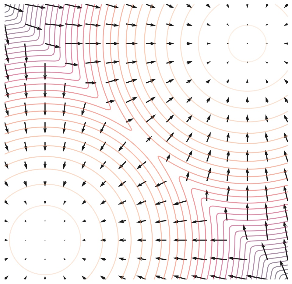
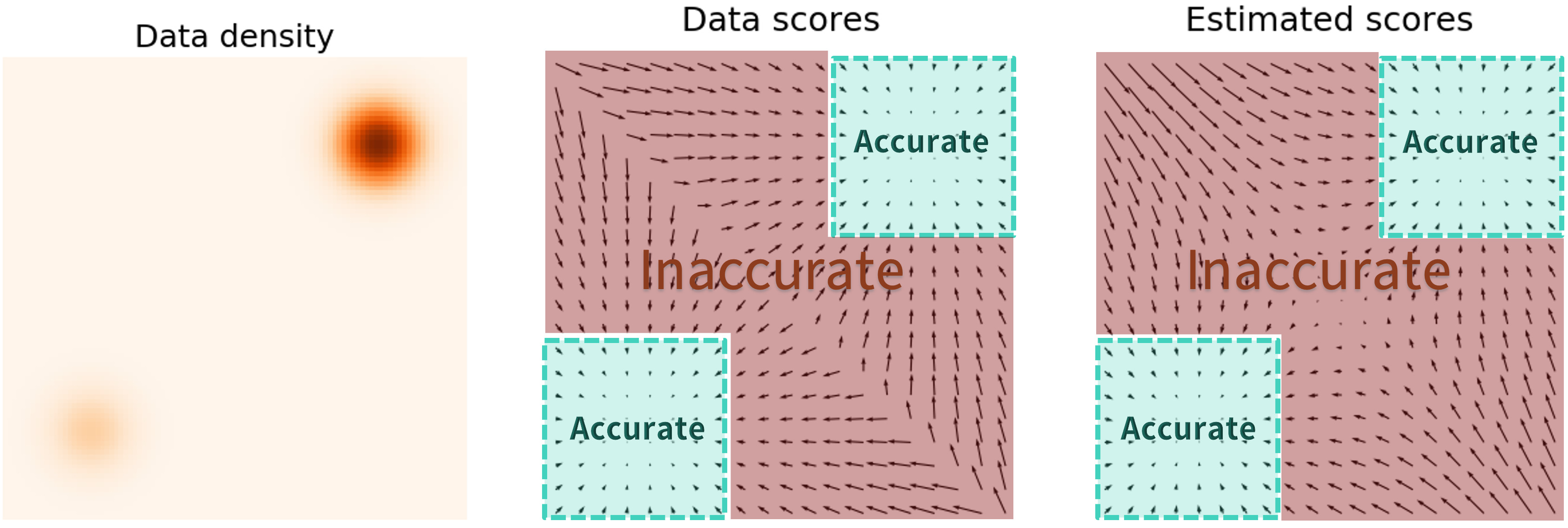
2. Low Coverage of Data Space ($s_{\theta }{\left(x\right)}^2$); Our model is not trained on input from the entire space (of course, we train on some data) so when we have input that come from random position outside data space that we trained on, model will be inaccurate in other word model don’t know correct direction, you can see that estimated scores are only accurate in high density regions (score point towards center).

Note: Why ${\nabla }_x{s}_{\theta }\left(x\right)$ is computable (but expensive) while $Z_{\theta }=\int e^{-f_{\theta }(\mathbf{x})}\mathrm{d}\mathbf{x}$ is not computable ? Answer: Integration is total area under the curve so we must compute integral over the entire input of $e^{-f_{\theta }(x)}$ which have high dimensional in other hand differential only take specific point $x$.

Noise Perturbation

To overcome Low Coverage of Data Space problem; We just add some Gaussian noise to data point

$$\tilde{x}=x+ϵ$$

where

$$ϵ\sim \mathcal{N}(0,{\sigma }^{2}I)$$

Now we denote our pdf as (new noise-perturbed pfd is depending on $\sigma$ which is noise level)

$$p(x)\stackrel{\mathrm{noise}}{\to }{p}_{\sigma }(\tilde{x})$$

and we train Noise Perturbed Objective

$$\frac{1}{2}{\mathbb{E}}_{p_{\sigma }(\tilde{x})}[\Vert {\nabla }_{\tilde{x}}\log p_{\sigma }(\tilde{x})-s_{\theta }(\tilde{x}){\Vert }_2^2]$$

here is what happens when we perturb a mixture of two Gaussian perturbed by additional Gaussian noise.

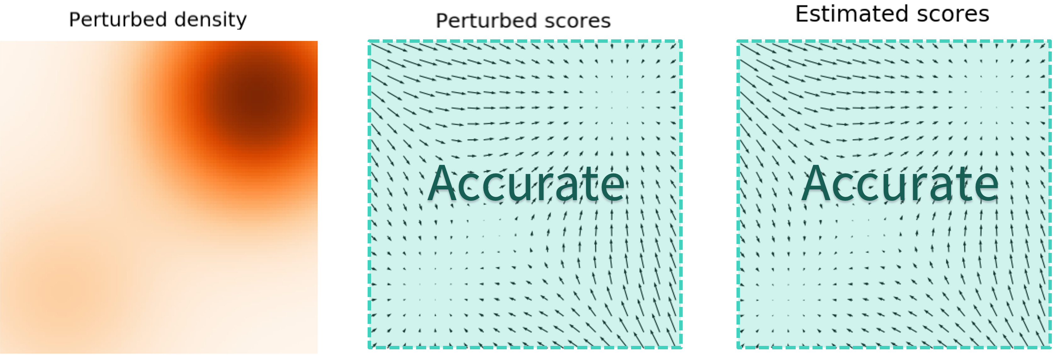
This improve the accuracy of model on low density region, but we still got tradeoff here

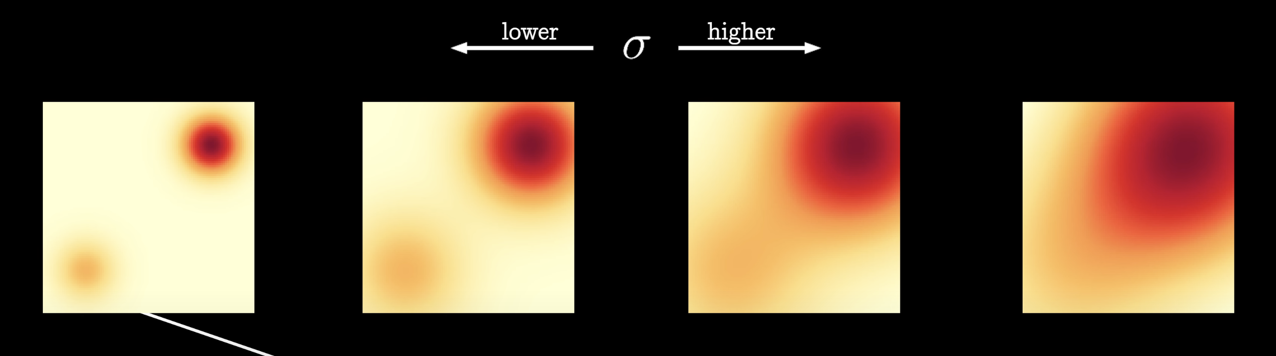
If we use high $\sigma$ (more noise):

• Cover more low density regions for better score estimation (resolve Low Coverage of Data Space).
• But it over-corrupts the data and alters it significantly from the original distribution

If we use low $\sigma$ (less noise):

• Facing Low Coverage of Data Space problem.
• Not over-corrupts the original data.

Connection to Denoising Autoencoders

someone found the connection between them and can overcome Expensive Training problem by reformulate score-matching objective from

$$\frac{1}{2}{\mathbb{E}}_{p_{\sigma }(\tilde{x})}[\Vert {\nabla }_{\tilde{x}}\log p_{\sigma }(\tilde{x})-s_{\theta }(\tilde{x}){\Vert }_2^2]$$

to this:

$$\frac{1}{2}{\mathbb{E}}_{\mathbf{x}\sim p(\mathbf{x}),\tilde{\mathbf{x}}\sim p_{\sigma }(\tilde{\mathbf{x}}|\mathbf{x})}[||s_{\theta }(\tilde{\mathbf{x}})-{\nabla }_{\tilde{\mathbf{x}}}\log p_{\sigma }(\tilde{\mathbf{x}}|\mathbf{x})|{|}_2^2]$$

This is huge, since normally in score-matching objective we don’t know $p_{\sigma }(\tilde{x})$ so we can’t compute ${\nabla }_{\tilde{x}}\log p_{\sigma }(\tilde{x})$, we do some math as describe above, and we got Expensive Training problem, but with this new objective we just need to know $p_{\sigma }(\tilde{\mathbf{x}}|\mathbf{x})$ and we know that in denoising autoencoders!

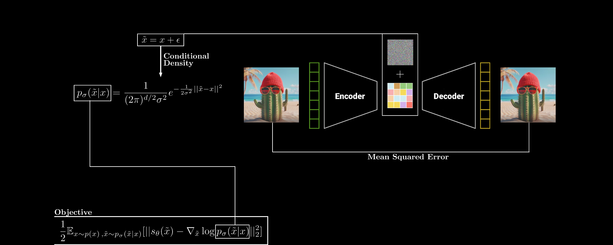
We just need to find $p_{\sigma }(\tilde{x}|x)$ by using Multivariate Gaussian distribution then compute ${\nabla }_{\tilde{\mathbf{x}}}\log p_{\sigma }(\tilde{\mathbf{x}}|\mathbf{x})$ and our new objective is to minimize this:

$$\frac{1}{2}{\mathbb{E}}_{x\sim p(x)},\tilde{x}\sim p_{\sigma }(\tilde{x}|x)[\left|\right|s_{\theta }\left(\tilde{x}\right)+\frac{1}{{\sigma }^2}ϵ\left|{|}_2^2\right]$$

This is beautiful, $\frac{1}{{\sigma }^2}ϵ$ is noise that we add to input and model need to predict $s_{\theta }(\tilde{x})=-\frac{1}{{\sigma }^2}ϵ$ in other word model need to predict direction(score) that back to original data point.

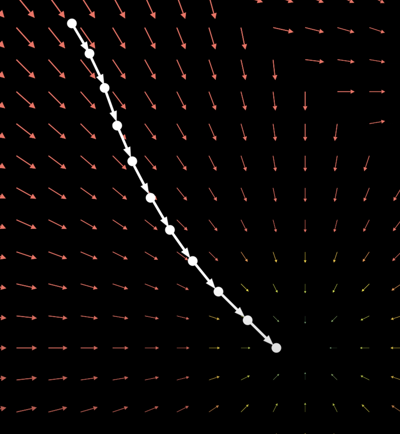
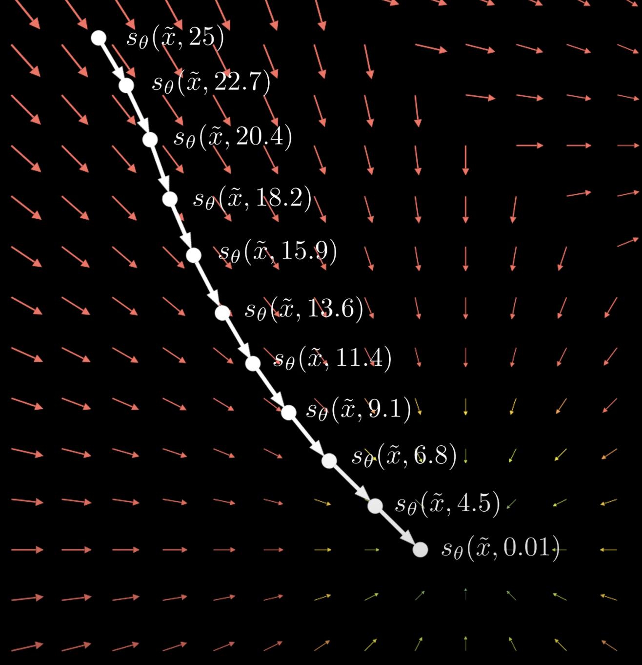
How to generate new sample ?

After training our score-based model we can do get denoise sample by iteratively predict new direction using Langevin Dynamics Sampling:

$$\begin{array}{c}{\tilde{x}}_{i+1}\leftarrow {\tilde{x}}_i+\alpha \cdot s_{\theta }(\widetilde{x_i})+\sqrt{2\alpha }\cdot ϵ\\ i=0,1,\cdot \cdot \cdot ,K\end{array}$$

At each step, we update the current sample ${\tilde{x}}_i$ by adding the product of a small step size $\alpha$ and the estimated score $s_{\theta }({\tilde{x}}_i)$. We also add the term $\sqrt{2\alpha }ϵ$ to introduce noise, which prevents all samples from collapsing to a single point. So our sample will become closer to data manifold.

Multiple Noise Perturbation

Recall that in Low Coverage of Data Space problem we have tradeoff when select $\sigma$, to achieve the best of both worlds, we use multiple scales of noise perturbations simultaneously.

We start from pre-specify $\sigma$ between $[0.01,25]$ which have total length $L$ with increasing standard deviations ${\sigma }_1<{\sigma }_2<\cdots <{\sigma }_L$ now got:

$$\tilde{x}=x+ϵ$$

where

$$\begin{array}{c}ϵ\sim \mathcal{N}(0,{\sigma }_i^{2}I)\\ i=1,2,\dots ,L\end{array}$$

now ${\sigma }_i$ is difference noise, and we add those noise as model input to give more information to model

$$s_{\theta }(\tilde{x},i)$$

and jointly train model for all noises

$$\sum _{i=1}^L\lambda (i){\mathbb{E}}_{p_{{\sigma }_i}(\mathbf{x})}[\Vert {\nabla }_{\mathbf{x}}\log p_{{\sigma }_i}(\mathbf{x})-{\mathbf{s}}_{\theta }(\mathbf{x},i){\Vert }_2^2]$$

After model is trained, we can use same sample technique except we start with the largest noise $i=L,L-1,\dots ,1$ since we know that large noise help model in low density region, This method is called annealed Langevin dynamics, also model that trained on difference noised scales is called Noise Conditional Score Networks (NCSNs).

In first paper they use 1000 noise scales.

Link to Stochastic Process

What is SDEs

How score-matching link to SDEs

In Multiple Noise Perturbation we use 1000 scales but If we want to cover as much noise scale as possible like 0.001 very small scale to very large scale like $\infty$ we no longer can write as discrete scale anymore (i.e., 1, 2, …, 1000 scales) it will be much better If we turn into function of time $X(t)$ where $t$ is time that control noise added to image (like control scale), so $X(t)$ is also known as Stochastic Process, how?

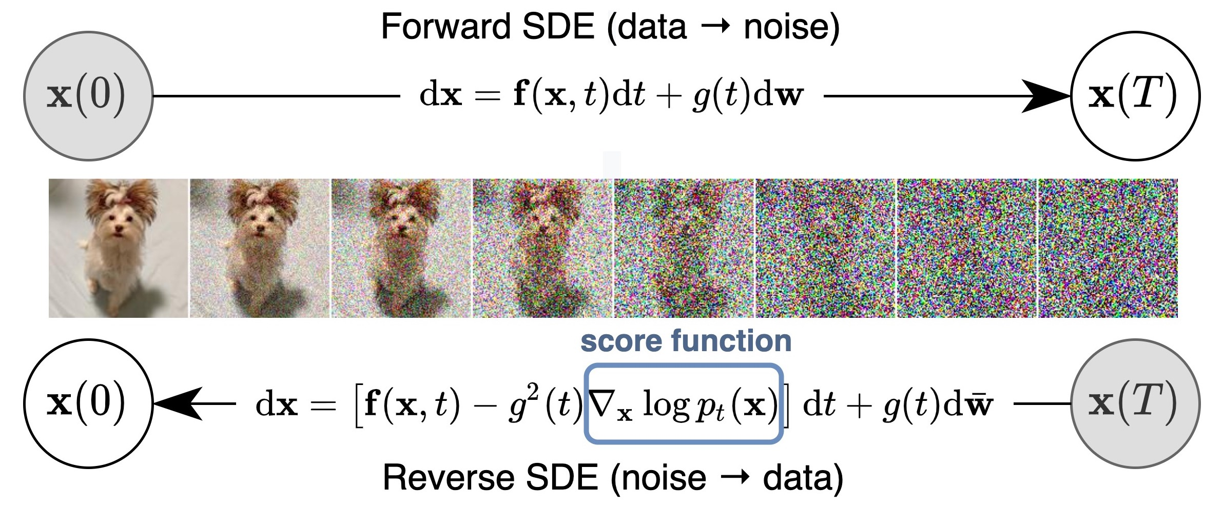
1. We start at our added noise data:

$$\tilde{x}=x+ϵϵ\sim \mathcal{N}(0,{\sigma }_i^{2}I)$$

2. Compare to SDEs equation

$$d{X}_t=\underset{deterministic(Drift)}{\underbrace{f(t,X_t)dt}}+\underset{stochastic(Diffusion)}{\underbrace{\sigma (t,X_t)d{W}_t}}$$

3. You can see that change in $x$ is just by adding noise $(ϵ)$ in other word change in $x$ only influence by stochastic term. We can write SDEs as:

$$dx=\sigma (t,X_t)d{W}_t$$

4. We know that stochastic term (noise that we add) is only change with time $t$ so we can remove input $X_t$. Now we can write SDEs as:

$$dx=\sigma (t)d{W}_t$$

5. If we got forward SDE, we can get reverse SDE:

$$\mathrm{d}x=[f(x,t)-g^2(t)\underset{scorefunction}{\underbrace{{\nabla }_x\log p_{\sigma }(x)}}]\mathrm{d}t+g(t)\mathrm{d}{W}_t$$

you can see that it use score function to reverse

Note that in many diffusion model will have technique to add noise differently, so detail in above step is not exactly the same, but idea and step is the same.

This method offers several advantages over using multiple discrete noise levels:

1. Continuous noise handling
2. Improved generalization
3. More accurate score estimation
4. Better sampling through continuous annealing
5. Flexibility in designing the noise schedule
6. Closer connection to the underlying data distribution

Summary

Score-function

The score function, by definition, gives you the gradient of the log probability density function at a given point. In other words, it tells you the direction in which the data density increases most steeply. Using just the score function, you can:

• Guide Sampling:
  By following the gradient directions (e.g., via Langevin dynamics), you can iteratively refine a random noise input into a sample that resembles data drawn from the target distribution.
• Denoising:
  In tasks like denoising, the score function indicates how to adjust a noisy input to move it toward higher probability regions, effectively “cleaning” the data.
• Solve Inverse Problems:
  The gradient information can be used to guide optimization processes to recover or reconstruct signals from corrupted or incomplete data.

They can be applied to both audio and images

Example Image Generation

Code for this example.

If we want to generate image (new sample), we all know that score-function alone only give direction at given point, so we need to do sampling to make new sample before we link to SDE we use Langevin Dynamics Sampling but after we link to SDE we can use reverse SDE instead.

Steps:

1. Define how we perturb our data (add noise to sample), in this example we use

$$\tilde{x}=x+ϵϵ\sim \mathcal{N}(0,{\sigma }^{2}I)$$

2. Define forward SDE from step (1) using forward SDE formula. In this case we got

$$d\mathbf{x}(t)={\sigma }^{t}d\mathbf{w}(t),t\in [0,1]$$

3. Solve forward SDE to get conditional probability, which will be plug into loss function later.
4. Plug conditional probability from step (2) into loss function.
5. Train score-based model using loss from (4).
6. After trained model, we create new sample (image) using these methods.

Other diffusion paper (e.g. DDPM, DDIM) design step (1) differently.

New loss function

Recall this loss function.

$$\mathcal{L}(\theta ;\sigma )=\frac{1}{2}{\mathbb{E}}_{\mathbf{x}\sim p(\mathbf{x}),\tilde{\mathbf{x}}\sim p_{\sigma }(\tilde{\mathbf{x}}|\mathbf{x})}[||s_{\theta }(\tilde{\mathbf{x}})-{\nabla }_{\tilde{\mathbf{x}}}\log p_{\sigma }(\tilde{\mathbf{x}}|\mathbf{x})|{|}_2^2]$$

this loss only use one noise level $(\sigma )$, from this section we learned that we need to train with multiple noise and this link to SDEs, so loss become

$$\mathcal{L}(\theta )=\underset{\theta }{\min }{\mathbb{E}}_{t\sim \mathcal{U}(0,T)}[\lambda (t){\mathbb{E}}_{\mathbf{x}(0)\sim p_0(\mathbf{x})}{\mathbf{E}}_{\mathbf{x}(t)\sim p_{0t}(\mathbf{x}(t)\mid \mathbf{x}(0))}[\Vert s_{\theta }(\mathbf{x}(t),t)-{\nabla }_{\mathbf{x}(t)}\log p_{0t}(\mathbf{x}(t)\mid \mathbf{x}(0)){\Vert }_2^2]]$$

These are changes:

1. Replace $x$ with stochastic process $x(t)$: $x(t)$ means noisy image at time $t$ while $x(0)$ is original image.
2. Replacing fixed $\sigma$ with time $t$: $t$ becomes the parameter controlling the noise level range from 0 (original image) to $T$ (noisy image). (recall this image)
3. Making noise distribution time-dependent: $p_{\sigma }(\tilde{x}|x)$ becomes $p_{0t}(x(t)|x(0))$.
4. Making the score model time-dependent: $s_{\theta }(\tilde{x})$ becomes $s_{\theta }(x(t),t)$.
5. Averaging the loss over different times (noise levels): Introducing ${\mathbb{E}}_{t\sim \mathcal{U}(0,T)}$
6. Weighting function $\lambda (t)$: Added to solve this problem

Build Time-Dependent Score-Based Model

Can be any architecture as long as input and output have same dimension, but effective one is U-net. Our model ideally produces $s_{\theta }(\mathbf{x}(t),t)$ so, input is $x$ (image) and $t$ (time or noise level) but how can we make model understand $t$ ?

Recall from link to SDEs section we know that $t$ is time in stochastic process which as $t$ increase noise added to image, to make model understand time $t$ the easiest way is just adding $t$ to every intermediate layer in U-net, but

1. we can’t code time as 0,1,2,..T, since $t$ is continuous in $[0,T]$
2. we can’t add single integer like 0,1,...,T we must represent time $t$ as vector instead, since neural network won’t learn much from single integer.

To solve these problems we must create projection function that can map any time $t$ (continuous) to higher dimension vector so we can add this vector to U-net, and it can learn time $t$ information, but what projection function we should use ?

To create such a projection function we must do like this:

1. In order to convert 1D time $t$ to high-dimension
   1. Create fixed random N-dimension vector.
   2. We can multiply any time $t$ with that vector.
   3. We will get vector that represent time $t$, difference $t$ will always have difference vector.
2. From (1) is just linear function this is not enough, since time can be complex and nonlinear. We further use Fourier features which is better to capture complex function, it is crucial that they are designed to be sufficiently expressive to encode the temporal information effectively.
3. what I mean is our projection function return $[\sin (2\pi \vec{x}),\cos (2\pi \vec{x})]$ where $\vec{x}$ is vector from (1).

Note: Projection means mapping data into a new space.

Lastly we normalize output of network by $\frac{1}{\sqrt{\text{variance}}}$ reason here.

Create new sample

Recall that for any SDE of the form

$$d\mathbf{x}=\mathbf{f}(\mathbf{x},t)dt+g(t)d\mathbf{w}$$

the reverse-time SDE is given by

$$d\mathbf{x}=[\mathbf{f}(\mathbf{x},t)-g(t{)}^2{\nabla }_{\mathbf{x}}\log p_t(\mathbf{x})]dt+g(t)d\bar{\mathbf{w}}$$

Since we have chosen the forward SDE to be

$$d\mathbf{x}={\sigma }^{t}d\mathbf{w},t\in [0,1]$$

The reverse-time SDE is given by

$$d\mathbf{x}=-{\sigma }^{2t}{\nabla }_{\mathbf{x}}\log p_t(\mathbf{x})dt+{\sigma }^{t}d\bar{\mathbf{w}}$$

To sample from our time-dependent score-based model $s_{\theta }(\mathbf{x},t)$, we first draw a sample from the prior distribution $p_1\approx \mathbf{N}(\mathbf{x};0,\frac{1}{2}({\sigma }^2-1)\mathbf{I})$, and then solve the reverse-time SDE with numerical methods.

1. Sampling with Numerical SDE Solvers (Euler–Maruyama)

For an SDE of the form

$$d\mathbf{x}=\mathbf{f}(\mathbf{x},t)dt+g(t)d\mathbf{w}$$

the Euler–Maruyama update rule is

$${\mathbf{x}}_{t+\Delta t}={\mathbf{x}}_t+\mathbf{f}({\mathbf{x}}_t,t)\Delta t+g(t)\sqrt{\Delta t}\mathbf{z}$$

where $\mathbf{z}$ is a sample from a standard normal distribution, $\mathbf{z}\sim \mathcal{N}(0,\mathbf{I})$ In the context of the reverse-time SDE, the method approximates

$$d\mathbf{x}=-{\sigma }^{2t}{s}_{\theta }(\mathbf{x},t)dt+{\sigma }^{t}d\bar{\mathbf{w}}$$

with the discretized iteration:

$${\mathbf{x}}_{t-\Delta t}=\underset{Drift}{\underbrace{{\mathbf{x}}_t+{\sigma }^{2t}{s}_{\theta }({\mathbf{x}}_t,t)\Delta t}}+\underset{Diffusion}{\underbrace{{\sigma }^t\sqrt{\Delta t}{\mathbf{z}}_t}}$$

• $s_{\theta }(\mathbf{x},t)\approx {\nabla }_{\mathbf{x}}\log p_t(\mathbf{x})$ is the estimated score function.
• $g(t)$ is the diffusion coefficient.
• $\Delta t$ is the time step.
• ${\mathbf{z}}_t\sim \mathcal{N}(0,\mathbf{I})$ is Gaussian noise.

We can loop this to generate new sample

2. Sampling with Predictor-Corrector Methods

We combine Predictor (Euler–Maruyama) with Corrector (Langevin MCMC). Recall the classical Langevin MCMC update is given by

$${\mathbf{x}}_{i+1}={\mathbf{x}}_i+ϵ{\nabla }_{\mathbf{x}}\log p({\mathbf{x}}_i)+\sqrt{2ϵ}{\mathbf{z}}_i$$

but instead of try to get next time step from this, we refine current time step and use Euler–Maruyama to get next time step instead, so Corrector update is

$$\mathbf{x}\leftarrow \mathbf{x}+ϵs_{\theta }(\mathbf{x},t)+\sqrt{2ϵ}\mathbf{z}$$

this is detail of how to select step size $ϵ$, then after we refine using Corrector, we use Predictor to get next time step. In summary:

1. Refines the sample using Langevin MCMC (corrector step) to reduce discretization error.
2. Propagates the refined sample using an Euler–Maruyama update (predictor step).

3. Sampling with Numerical ODE Solvers

In this paper they found that, For any Forward SDE of the form

$$d\mathbf{x}=\mathbf{f}(\mathbf{x},t)dt+g(t)d\mathbf{w}$$

and have Reverse SDE:

$$d\mathbf{x}=[\mathbf{f}(\mathbf{x},t)-g(t{)}^2{\nabla }_{\mathbf{x}}\log p_t(\mathbf{x})]dt+g(t)d\bar{\mathbf{w}}$$

It turns out that Reverse SDE have an associated ODE

$$d\mathbf{x}=[\mathbf{f}(\mathbf{x},t)-\frac{1}{2}g(t{)}^2{\nabla }_{\mathbf{x}}\log p_t(\mathbf{x})]dt$$

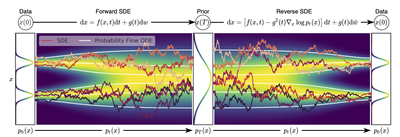
which is known as the probability flow ODE. Despite being deterministic (i.e., without the random noise term), this ODE has trajectories whose marginal distributions $p_t(\mathbf{x})$ match those of the original SDE. This means that if you solve this ODE from time $T$ to $0$, starting with a sample from $p_T$, you’ll obtain a sample from $p_0$ (typically the data distribution).

Below is a schematic figure showing how trajectories from this probability flow ODE differ from SDE trajectories, while still sampling from the same distribution.

Therefore, we can start from a sample from $p_T$, integrate the ODE in the reverse time direction, and then get a sample from $p_0$. In particular, for the SDE in our running example, we can integrate the following ODE from $t=T$ to $0$ for sample generation

$$d\mathbf{x}=-\frac{1}{2}{\sigma }^{2t}{s}_{\theta }(\mathbf{x},t)dt$$